Phần 3: Ví dụ minh họa cho mô hình SVM
Xây dựng một bộ dữ liệu và đường phân cách đơn giản để thực nghiệm.
import numpy as np
import pandas as pd
from matplotlib import pyplot as plt
import seaborn as sns
sns.set()

from sklearn.svm import SVC
from cvxopt import matrix as cvxopt_matrix
from cvxopt import solvers as cvxopt_solvers
#Data set
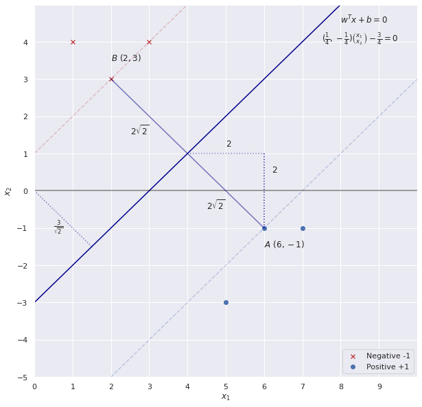
x_neg = np.array([[3,4],[1,4],[2,3]])
y_neg = np.array([-1,-1,-1])
x_pos = np.array([[6,-1],[7,-1],[5,-3]])
y_pos = np.array([1,1,1])
x1 = np.linspace(-10,10)
x = np.vstack((np.linspace(-10,10),np.linspace(-10,10)))
#Data for the next section
X = np.vstack((x_pos, x_neg)) #Matrix for next calculating
y = np.concatenate((y_pos,y_neg))
#Parameters guessed by inspection
w = np.array([1,-1]).reshape(-1,1)
b = -3
#Plot
fig = plt.figure(figsize = (10,10))
plt.scatter(x_neg[:,0], x_neg[:,1], marker = 'x', color = 'r', label = 'Negative -1')
plt.scatter(x_pos[:,0], x_pos[:,1], marker = 'o', color = 'b',label = 'Positive +1')
plt.plot(x1, x1 - 3, color = 'darkblue')
plt.plot(x1, x1 - 7, linestyle = '--', alpha = .3, color = 'b')
plt.plot(x1, x1 + 1, linestyle = '--', alpha = .3, color = 'r')
plt.xlim(0,10)
plt.ylim(-5,5)
plt.xticks(np.arange(0, 10, step=1))
plt.yticks(np.arange(-5, 5, step=1))
#Lines
plt.axvline(0, color = 'black', alpha = .5)
plt.axhline(0,color = 'black', alpha = .5)
plt.plot([2,6],[3,-1], linestyle = '-', color = 'darkblue', alpha = .5 )
plt.plot([4,6],[1,1],[6,6],[1,-1], linestyle = ':', color = 'darkblue', alpha = .5 )
plt.plot([0,1.5],[0,-1.5],[6,6],[1,-1], linestyle = ':', color = 'darkblue', alpha = .5 )
#Annotations
plt.annotate(s = '$A \ (6,-1)$', xy = (5,-1), xytext = (6,-1.5))
plt.annotate(s = '$B \ (2,3)$', xy = (2,3), xytext = (2,3.5))#, arrowprops = {'width':.2, 'headwidth':8})
plt.annotate(s = '$2$', xy = (5,1.2), xytext = (5,1.2) )
plt.annotate(s = '$2$', xy = (6.2,.5), xytext = (6.2,.5))
plt.annotate(s = '$2\sqrt{2}$', xy = (4.5,-.5), xytext = (4.5,-.5))
plt.annotate(s = '$2\sqrt{2}$', xy = (2.5,1.5), xytext = (2.5,1.5))
plt.annotate(s = '$w^Tx + b = 0$', xy = (8,4.5), xytext = (8,4.5))
plt.annotate(s = '$(\\frac{1}{4},-\\frac{1}{4}) \\binom{x_1}{x_2}- \\frac{3}{4} = 0$', xy = (7.5,4), xytext = (7.5,4))
plt.annotate(s = '$\\frac{3}{\sqrt{2}}$', xy = (.5,-1), xytext = (.5,-1))
#Labels and show
plt.xlabel('$x_1$')
plt.ylabel('$x_2$')
plt.legend(loc = 'lower right')
plt.show()
Giải bài toán SVM (Hard Margin):
Ta có bài toán tối ưu của SVM như sau:
\[\underset{\alpha}{\operatorname{argmin}} \frac{1}{2} \sum_{n=1}^N \sum_{m=1}^N y_n y_m \alpha_n \alpha_m x_n^T x_m - \sum_{n=1}^N \alpha_n\]Ta có thể giải bài toán này với dạng Quadratic với bài toán tổng quát như sau:
\[\underset{\alpha}{\operatorname{argmin}} \frac{1}{2} x^T P x + q^T x \\ \text{subject to: } Gx \leq h \\ Ax = b ~~~~ (*)\]Ta sẽ xây dựng các tham số để giải bài toán SVM bằng QP như sau:
Gọi $H$ là ma trận kích thước $mxm$ với $H_{n, m} = y_n y_m x_n^T x_m$
Từ đây ta sẽ có bài toán tối ưu cho SVM được viết như sau:
\[\underset{\alpha}{\operatorname{argmin}} \frac{1}{2} \alpha^T H \alpha -1^T \alpha \\ \text{subject to: } -\alpha_n \leq 0 \\ y^T \alpha = 0\]Ta gán lại một số tham số tiện cho việc sử dụng hàm tối ưu trong biểu thức (*):
- Ma trận P là ma trận H
- Vector q là vector kích thước $mx1$ với các giá trị đều là -1.
- Ma trận G là ma trận đường chéo kích thước $mxm$ với các giá trị trên đường chéo là -1. Để ta áp dụng ràng buộc cho $G\alpha \leq 0$
- Vector h là vector 0 kích thước $mx1$
- Vector A là vector của các giá trị y.
- b là một scalar giá trị bằng 0.
#Initializing values and computing H. Note the 1. to force to float type
m,n = X.shape
y = y.reshape(-1,1) * 1.
X_dash = y * X
H = np.dot(X_dash , X_dash.T) * 1. #calculating H matrix

#Converting into cvxopt format
P = cvxopt_matrix(H)
q = cvxopt_matrix(-np.ones((m, 1)))
G = cvxopt_matrix(-np.eye(m))
h = cvxopt_matrix(np.zeros(m))
A = cvxopt_matrix(y.reshape(1, -1))
b = cvxopt_matrix(np.zeros(1))

#Setting solver parameters (change default to decrease tolerance)
cvxopt_solvers.options['show_progress'] = False
cvxopt_solvers.options['abstol'] = 1e-10
cvxopt_solvers.options['reltol'] = 1e-10
cvxopt_solvers.options['feastol'] = 1e-10

#Run solver
sol = cvxopt_solvers.qp(P, q, G, h, A, b)
alphas = np.array(sol['x'])
Tính toán $w, b$ dựa trên các giá trị $\alpha_n$
#w parameter in vectorized form
w = ((y * alphas).T @ X).reshape(-1,1)

#Selecting the set of indices S corresponding to non zero parameters
S = (alphas > 1e-4).flatten()

#Computing b
b = y[S] - np.dot(X[S], w)

#Display results
print('Alphas = ',alphas[alphas > 1e-4])
print('w = ', w.flatten())
print('b = ', b[0])
Alphas =  [0.0625     0.06249356]
w =  [ 0.24999356 -0.25000644]
b =  [-0.74996781]
So sánh kết quả $w, b$ với sklearn
clf = SVC(C = 1e10, kernel = 'linear') # With a very large C for hard margin
clf.fit(X, y.ravel())

print('w = ',clf.coef_)
print('b = ',clf.intercept_)
print('Indices of support vectors = ', clf.support_)
print('Support vectors = ', clf.support_vectors_)
print('Number of support vectors for each class = ', clf.n_support_)
print('Coefficients of the support vector in the decision function = ', np.abs(clf.dual_coef_))
w =  [[ 0.25 -0.25]]
b =  [-0.75]
Indices of support vectors =  [5 0]
Support vectors =  [[ 2.  3.]
 [ 6. -1.]]
Number of support vectors for each class =  [1 1]
Coefficients of the support vector in the decision function =  [[0.0625 0.0625]]
Giải bài toán SVM-Soft Margin
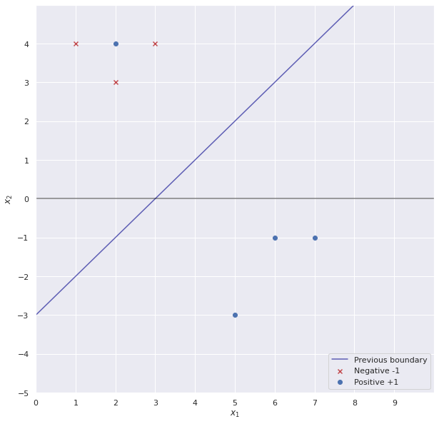
Chúng ta sẽ chỉnh sửa 1 số dữ liệu để dữ liệu chúng ta không còn linear separablity. Để tiện cho việc tìm kết quả, ta chỉ sửa lại 1 điểm dữ liệu và đường phân tách vẫn giữ nguyên.
x_neg = np.array([[3,4],[1,4],[2,3]])
y_neg = np.array([-1,-1,-1])
x_pos = np.array([[6,-1],[7,-1],[5,-3],[2,4]])
y_pos = np.array([1,1,1,1])
x1 = np.linspace(-10,10)
x = np.vstack((np.linspace(-10,10),np.linspace(-10,10)))


fig = plt.figure(figsize = (10,10))
plt.scatter(x_neg[:,0], x_neg[:,1], marker = 'x', color = 'r', label = 'Negative -1')
plt.scatter(x_pos[:,0], x_pos[:,1], marker = 'o', color = 'b',label = 'Positive +1')
plt.plot(x1, x1  - 3, color = 'darkblue', alpha = .6, label = 'Previous boundary')
plt.xlim(0,10)
plt.ylim(-5,5)
plt.xticks(np.arange(0, 10, step=1))
plt.yticks(np.arange(-5, 5, step=1))

#Lines
plt.axvline(0, color = 'black', alpha = .5)
plt.axhline(0,color = 'black', alpha = .5)


plt.xlabel('$x_1$')
plt.ylabel('$x_2$')

plt.legend(loc = 'lower right')
plt.show()

#New dataset (for later)
X = np.array([[3,4],[1,4],[2,3],[6,-1],[7,-1],[5,-3],[2,4]] )
y = np.array([-1,-1, -1, 1, 1 , 1, 1 ])
Với bài toán tối ưu cho SVM soft-margin, ta chỉ cần thêm ràng buộc $0 \leq \alpha_n \leq C$.
Bài toán tối ưu như sau:
\[\underset{\alpha}{\operatorname{argmin}} \frac{1}{2} \alpha^T H \alpha -1^T \alpha \\ \text{subject to: } -\alpha_n \leq 0 \\ 0 \leq \alpha_n \leq C \\ y^T \alpha = 0\]Ta sẽ sửa lại 1 số giá trị cho việc thêm vào ràng buộc $0 \leq \alpha \leq C$ bằng cách chỉnh sửa ma trận G và vector h như sau (giả sử như ta dùng 2 chiều để biểu diễn ra các $\alpha$):
\[G = \begin{bmatrix} -1 & 0\\ 0 & -1\\ 1 & 0\\ 0 & 1 \end{bmatrix} \\ h = \begin{bmatrix} 0\\ 0\\ C\\ C \end{bmatrix}\]Từ đó các $-\alpha_n \leq 0$ và $0 \leq \alpha_n \leq C$.
#Initializing values and computing H. Note the 1. to force to float type
C = 10 #Hyperparameter for C
m,n = X.shape
y = y.reshape(-1,1) * 1.
X_dash = y * X
H = np.dot(X_dash , X_dash.T) * 1.

#Converting into cvxopt format - as previously
P = cvxopt_matrix(H)
q = cvxopt_matrix(-np.ones((m, 1)))
G = cvxopt_matrix(np.vstack((np.eye(m)*-1,np.eye(m)))) #Create new G
h = cvxopt_matrix(np.hstack((np.zeros(m), np.ones(m) * C))) #Create new h
A = cvxopt_matrix(y.reshape(1, -1))
b = cvxopt_matrix(np.zeros(1))

#Run solver
sol = cvxopt_solvers.qp(P, q, G, h, A, b)
alphas = np.array(sol['x'])

#==================Computing and printing parameters===============================#
w = ((y * alphas).T @ X).reshape(-1,1)
S = (alphas > 1e-4).flatten()
b = y[S] - np.dot(X[S], w)

#Display results
print('Alphas = ',alphas[alphas > 1e-4])
print('w = ', w.flatten())
print('b = ', b[0])
Alphas =  [ 5.      6.3125  1.3125 10.    ]
w =  [ 0.25 -0.25]
b =  [-0.75]
So sánh kết quả $w, b$ với sklearn với soft-margin
clf = SVC(C = 10, kernel = 'linear')
clf.fit(X, y.ravel())

print('w = ',clf.coef_)
print('b = ',clf.intercept_)
print('Indices of support vectors = ', clf.support_)
print('Support vectors = ', clf.support_vectors_)
print('Number of support vectors for each class = ', clf.n_support_)
print('Coefficients of the support vector in the decision function = ', np.abs(clf.dual_coef_))
w =  [[ 0.25 -0.25]]
b =  [-0.75]
Indices of support vectors =  [0 2 3 6]
Support vectors =  [[ 3.  4.]
 [ 2.  3.]
 [ 6. -1.]
 [ 2.  4.]]
Number of support vectors for each class =  [2 2]
Coefficients of the support vector in the decision function =  [[ 5.      6.3125  1.3125 10.    ]]
Trong thực tế, việc implement các mô hình SVM ở thư viện có sẵn như sklearn sử dụng nhiều cách tối ưu khác nhau, không nhất thiết phải dùng Quadratic Programming (có thể sử dụng một số phương pháp khác như Sequential Minimal Optimization).
Tài liệu tham khảo
- Khóa Learning from Data của Caltech
- Ví dụ minh họa được lấy từ: https://xavierbourretsicotte.github.io/SVM_implementation.html
- https://machinelearningcoban.com/2017/04/09/smv/
- Document cho mô hình SVM: https://scikit-learn.org/stable/modules/svm.html và các practical usage cho việc chọn các tham số của SVM: https://scikit-learn.org/stable/modules/svm.html#tips-on-practical-use


Leave a comment